How to measure plasma and mitochondrial membrane potential in an unbiased manner
The assay comprises recording and analysis parts. You perform the recording on an arbitrary live-cell fluorescence microscope setup based on our protocols and publications. You use your own reagents or our reagents that will be available later. You perform image and data analysis in Image Analyst MKII. Purchased software license allows all analysis required to perform the analysis.
- Adherent or immobilized cell cultures in glass-bottomed microplates are amenable to the assay.
- To keep conditions as physiological as possible, we designed specialty assay media based on nonfluorescent culture media, where glucose, pyruvate, glutamine, and Ca2+ can be varied.
- A fluorescence time course is recorded in two channels, looking at tetramethylrhodamine methyl ester (TMRM) and FLIPR membrane potential probe (aka. PMPI) fluorescence using an arbitrary motorized microscope.
- During recording, cultures may be challenged multiple times by part-replacement of the potentiometric assay medium.
- The arbitrary time course recording is followed by a standardized
calibration paradigm. This allows calculation of millivolt values for
the entire time course by Image Analyst MKII for both ΔψP and ΔψM. Calibration
points for “complete calibration”:
- zero ΔψM
- stepwise increments of [K+]EC to depolarize ΔψP
- zero ΔψP
- Two cell type-specific geometric parameters are measured in separate experiments using confocal microscopy (or looked up from tables).
- Wet-bench assay protocols are available here.
- Image and data analysis is aided by an interactive protocol in Image Analyst Primer Window (see below).
The Potentiometric Assay - Experimental design and data analysis

Step 1: The potentiometric assay paradigm
The assay can be performed on any epifluorescence (suitable for low-light level time-lapse imaging), confocal or two-photon system. A prototype experiment is exemplified below using human pancreatic beta-cells (published in (26)). An arbitrary time course recording is followed by a standardized calibration paradigm. The calibrant cocktails have been described in (17), and their preparation in (61).
Step 2: Image Analysis
The mitochondrial membrane potential analysis can now be performed using an interactive protocol in the Primer Window by selecting Assays/Intensity and Ratio Measurements/ Mitochondrial membrane potential assay - worked example. Buttons in the protocol actually operate Image Analyst MKII.
Mitochondrial membrane potential assay - worked example - an interactive protocol
- Analysis protocol
-
Experimental Protocol
Link to: Absolute mitochondrial membrane potential measurement in β-cells
Image Processing
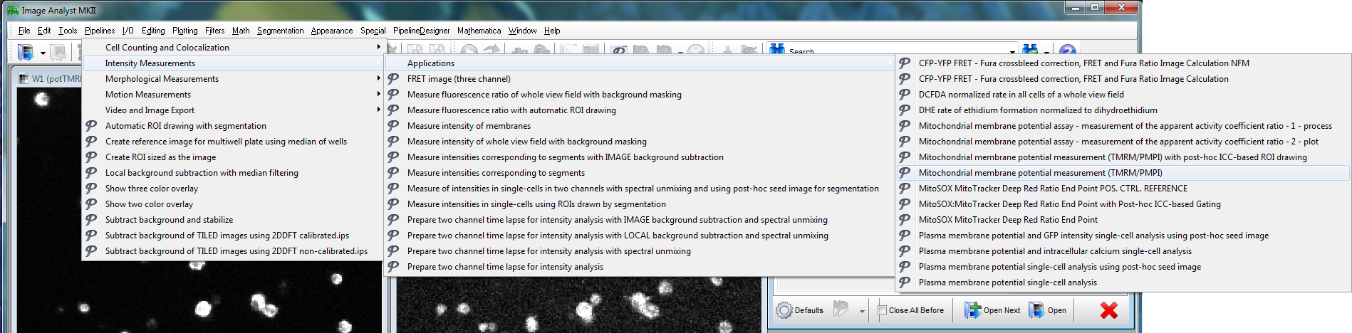
The pipelines used here can be accessed from the main menu: Pipelines/Intensity Measurements/Applications. Use the buttons below to activate the pipelines and perform the analysis:-
 Open the recording
by selecting all recorded files comprising the time lapse. For the
worked example select *.nd2 as file type in the Open dialog.
Open the recording
by selecting all recorded files comprising the time lapse. For the
worked example select *.nd2 as file type in the Open dialog. - Alternatively use multiple file selection in the Windows Explorer and drag-and-drop on the Image Analyst MKII. Note: check the correct order in the Files tab of the Multi-Dimensional Open dialog.
- Select the Pipelines/Intensity Measurements/
 Mitochondrial membrane potential assay
(TMRM/FLIPR)
Mitochondrial membrane potential assay
(TMRM/FLIPR) pipeline.
- Alternatively available pipelines:
- If the view field is contaminated by dead cells (bright FLIPR at the baseline) select: Pipelines/Intensity Measurements/Mitochondrial membrane potential assay (TMRM/FLIPR) with masking dead cells
- To analyze groups of cells, because individual cells
overlap or move during the assay select: Pipelines/Intensity Measurements/Mitochondrial membrane potential assay (TMRM/FLIPR) with masking dead cells - for groups of cells
- See other flavors of the assay pipeline supporting gating of single cells in Pipelines/Intensity Measurements/Applications.
- If the view field is contaminated by dead cells (bright FLIPR at the baseline) select: Pipelines/Intensity Measurements/
- Alternatively available pipelines:
- The default parameters of the pipeline have been configured to work with
this particular recording.
- Press the
 Run button
on the main toolbar or in the bottom of the Multi-Dimensional Open dialog.
Run button
on the main toolbar or in the bottom of the Multi-Dimensional Open dialog. - Observe the resultant images, and if ROIs are not as desired Adjust the pipeline and re-run.
- When the pipeline is executed, configure the Membrane Potential Calibration Wizard as given below.
- Calibration of multiple recordings (stage positions):
- When the Wizard is fully configured save the calibration
configuration using the
 button.
 - Set the pipeline parameter Membrane potential calibration action to Calibrate.
- Browse for the saved calibration configuration file at the Calibration configuration file name (*.ips) parameter.
- Set up saving to Excel using the Output Excel Data save file name (*.xlsx) parameter, by setting automatic file naming e.g. "=%LoadBaseName%_%LoadStageNumber%.xlsx", or alternatively configure a Prism file for data output.
- Use the pull down menu of the
Run button
to run the pipeline in all positions.
- When the Wizard is fully configured save the calibration
configuration using the
Membrane Potential Calibration Wizard
1. Calibration Method tab:
1.1. Choose the plasma membrane potential calibration method: “Complete with known kP (K-steps)”
1.2. Choose the mitochondrial membrane potential calibration method: “Complete”
2. Input/Output tab: the input images have been already selected by the pipeline.
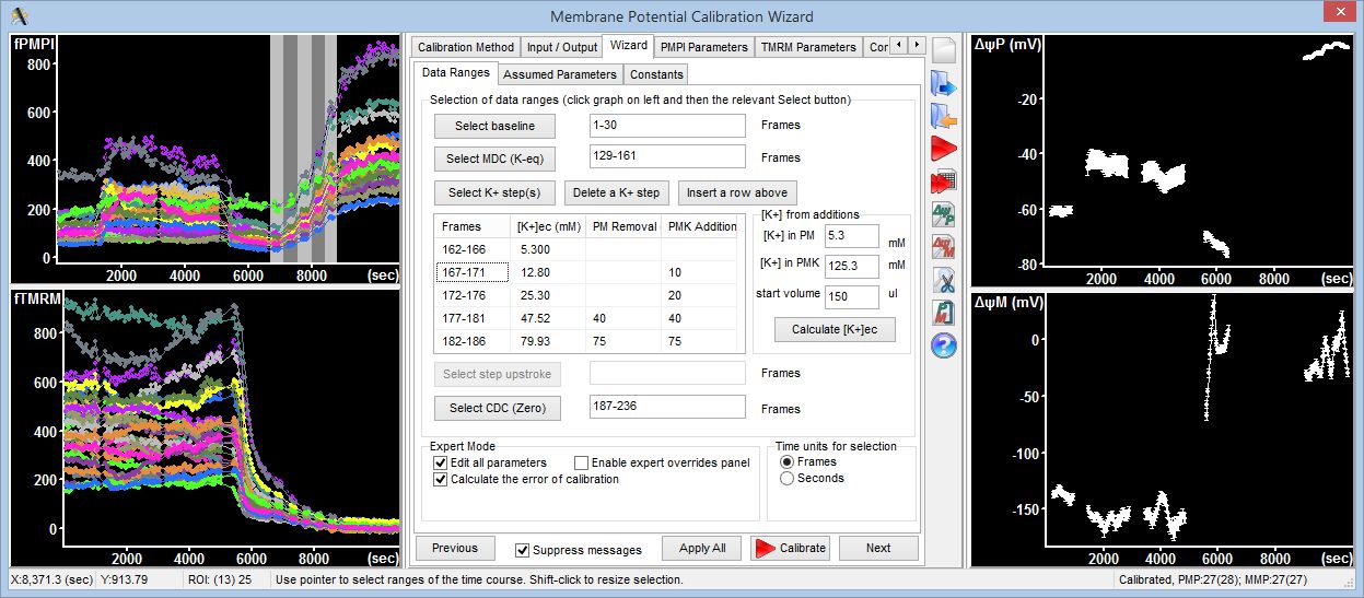
3. Wizard – Data Ranges tab:
3.1. Select baseline by pointing the range in one of the graphs on the left, and press the “Select baseline" button or alternatively 1-30 next to the “Select baseline" button.
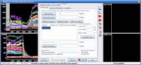
3.2. Select complete mitochondrial depolarization in the graph, and press the “Select MDC (K-eq)” button (135-169).
3.3. Select final complete depolarization in the graph, and press the “Select CDC (zero)” button (222-245).
3.4. Select the K+-steps, the five segments visible between the mitochondrial and complete depolarization in the top left graph, and press the “Select a K+ step(s)” button.
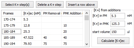
3.5. To calculate [K+] during K-steps, enter the K+ concentration in the potentiometric medium (PM), that was 5.3 mM and in the K-based potentiometric medium (PMK), that was 125.3 mM, and the medium volume (150 µl). The K-steps were performed by first adding 10 µl PMK to the assay well. Enter 10 to the second line and “PMK Addition” column in the K-steps table. This was followed by addition of 20 µl (enter it in the next line), then removal of 40 µl and addition of 40ul (in the next line enter 40 to the “PM Removal” column and 40 to the “PMK Addition” column. Finally 75 µl was removed and 75 µl was added (fifth line of the table). Press the “Calculate [K+]ec button”.
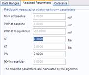
4. Wizard – Assumed Parameters tab: No action is required, use the default rate constant for FLIPR redistribution kP=0.38 s-1, and assume no significant non-K-permeability of the plasma membrane during K-steps by using the default PN=0.
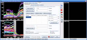
5. Wizard – Constants tab: set the cell specific parameters here:
5.1. VF (mitochondrion:cell volume fraction): use the Measurement of mitochondria:cell volume fraction (VF) protocol to measure this value using confocal microscopy, assume it based on literature. For the example data set it was measured to be 0.0772 ± 0.0016.
5.2. VFM (matrix:cell volume fraction): this value affects the results only little (because aR’ –see below- largely cancels its effects). The default is 0.8
5.3. aR’ (apparent activity coefficient ratio): use the Measurement of apparent activity coefficient ratio for TMRM (aR') protocol to measure this value using confocal microscopy. For the example data set it was measured to be 0.361 ± 0.005
5.4. Leave all other constants at their default values.
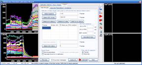
6. Press the
 Calibrate
button to perform the calibration. Note: not all cells in
the view field can be calibrated, therefore error messages will appear to
note this, unless “Suppress messages” in the
bottom of the Calibration Wizard is checked.
Calibrate
button to perform the calibration. Note: not all cells in
the view field can be calibrated, therefore error messages will appear to
note this, unless “Suppress messages” in the
bottom of the Calibration Wizard is checked.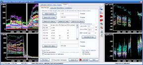
7. To save results
7.1 For Excel press
 and
and
7.2 Alternatively to record data to a Graphpad Prism file, first click File/Create New or Open Existing Prism File or the
 button in the Wizard. See more about saving to Excel or Prism here.
7.3 To directly access data right-click / ”Copy Plot Data” in the graphs on the graphs on the right.
8. To explore the results:
8.1. Use the
 and
and
 buttons
to see the regression analysis used to calculate calibration parameters
buttons
to see the regression analysis used to calculate calibration parameters8.2. Use the
 button
to see only the time course preceding the calibration steps.
button
to see only the time course preceding the calibration steps.8.3. Use the
 button
to see only those plasma membrane traces that also were successfully
calibrated for mitochondrial membrane potential. Press
again
to refresh the results.
button
to see only those plasma membrane traces that also were successfully
calibrated for mitochondrial membrane potential. Press
again
to refresh the results.8.4. Right-click / “Calculate Mean” to see mean±SE of all calibrated traces. Note: if the mean calculation is performed on the fluorescence traces on the left, then the mean data will be calibrated.
-
- Adjustments
-
1. Configuration of the pipeline:
- Set channel number associations for TMRM and FLIPR
- If not using local background subtraction, set frame-by-frame background subtraction as follows:
- The cells are very sparse Use background level of 50 percentile.
- The culture is subconfluent Use background level of 20 percentile.
- The culture is confluent Use background level of 5 percentile.
- Note: Percentiles below 5-10 may increase noise.
- For generic removal of inhomogeneous background use Local background subtraction by median rolling ball = Yes.
-
Run
the pipeline,
and observe the resultant ROIs. Adjust parameters if required and run pipeline again. Click the buttons below to adjust:
- Single cells are detected as multiple segments / Multiple cells are detected as single segments
- Turn segment welding on / off in addition, to address the above.
- Debris is detected as cells / Dimmer cells are missed
- Only bright debris is detected / Brightest areas are clipped or fused
- ROIs are smaller than cells / ROIs are too large or spilling over to background
2. Spectral unmixing
The analysis of TMRM/FLIPR recordings requires spectral unmixing. See related "Calculation of spectral unmixing coefficients for the ΔψM assay" interactive protocol in the Primer. The spectral unmixing coefficient matrix qualifies the configuration of the microscope, so it has to be re-measured if the relevant microscope configuration changes, but not for different specimens. The ratio of the two (TMRM and FLIPR) exposure times affects the coefficients, but a change exposure time can be accounted for by changing exposure correction parameters in the Spectral Unmixing function by editing the pipeline.
Enter the coefficient matrix as calculated.
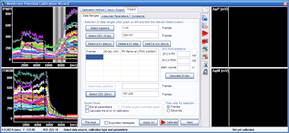
3. Quality control of the calibration:
3.1. Check “Calculate the error of calibration” in the Data ranges tab within the Wizard tab and press
.
Now the predicted error of the calibration is shown. Note:
optionally, check the “Suppress messages” on the bottom.3.2. Check “Edit all parameters”. Detailed lists of all parameters for FLIPR and TMRM calibration, common calibration constants, and error propagation parameters are shown in tabs appearing on the right of the Wizard tab on the top.
3.3. In the FLIPR parameters, set Quality control by propagated error of baseline to “Yes” and press
.
Traces with larger predicted error than set at the parameter below disappear
now. 3.4. In the TMRM parameters, set Quality control by propagated error of baseline to “Yes” and press
.
Traces with larger predicted error than set at the parameter below disappear
now. 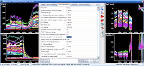
4. Using the Expert Mode: When the Edit all parameters checkbox is checked in the Data ranges tab within the Wizard tab, all parameters of the calibration algorithms can be directly accessed in the tabs appearing on the right of the Wizard tab. These can be used alternatively to the Wizards tab to enter any of the parameters. Use the “Fill in Range(s)” button to automatically enter a range from the selection made in the right graphs.
5. Fine tuning the calibration
5.1. Switch to the “Constants” tab, for this the “Edit all parameters” needs to be checked in the “Wizard” tab.
5.2. To accommodate to the temporal resolution and noise of the recording, adjust the “Differentiation kernel width” to 11 frames. Larger width suppresses noise by providing more smoothing, but also smears fast changes.
5.3. Median filter for baseline, fft0 and fp0: if using the “Take maximum of CDC Range” in the “FLIPR Parameters” tab or “Take minimum of CDC Range” in the “TMRM Parameters” use this option to suppress noise affecting minimum and maximum calculations.
- Output
-
1. Output options
-
Excel: Click
in
the Wizard.
-
button in the Wizard. See more about saving to Excel or Prism here.
-
To directly access data right-click / ”Copy Plot Data” in the graphs on the graphs on the right.
2. Automation
2.1. Save an arbitrary calibration configuration using the
 button
in the Membrane Potential Calibration Wizard.
button
in the Membrane Potential Calibration Wizard.2.2. In the Pipeline Parameters (Main Window Parameter Bar; the “Mitochondrial membrane potential assay (TMRM/FLIPR)” pipeline is activated) click the “Calibration configuration file name (*.ips)” parameter, and click the button appearing at the end of the line. Select the saved calibration file.
2.3. If using Excel, to automate saving the results give a filename in the “Output Excel Data save file name (*.xlsx)” using the string parser, such as =%LoadBaseName%%LoadPositionNumber:2%.xlsx. See more about the string parser in the Main menu Help/”Help on Expression Evaluation”. Optionally give a path, or set the default path to be used in the Main menu Files/”Set Folder Locations”.
2.5. Use the pull down menu of the
 button
on the main toolbar or in the bottom of the Multi-Dimensional Open dialog to
select “Run pipeline … on all stage positions” or “Run pipeline … on partial
plate”.
button
on the main toolbar or in the bottom of the Multi-Dimensional Open dialog to
select “Run pipeline … on all stage positions” or “Run pipeline … on partial
plate”. -
Alternatively, select from a set of pre-configured pipelines in the main menu of Image Analyst MKII to process fluorescence time-lapse image recordings and automatically draw ROIs to extract fluorescence intensities. See tutorial image data for potentiometric image analysis here, and a video tutorial here.
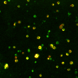
Left: Microscopic
view-field of TMRM (red) and FLIPR (green) fluorescence in
pancreatic beta-cells.
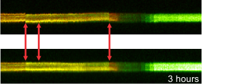
Right: Effect of channel alignment
and image stabilization of the time lapse, demonstrated by a
line scan
These image processing steps are included into the standard pre-processing pipelines for potentiometric calibrations.
Step 3: Calculation of millivolts using the Membrane Potential Calibration Wizard
The Membrane Potential Calibration Wizard guides the user through the calibration procedure. The user selects the experimental paradigm matching the recording, then points the ranges of calibrant additions on the fluorescence time courses, and finally enters required additional parameters. In the complete calibration paradigm only volumes of K+-based medium additions are required to perform the calibration.
- Complete (temporally resolved K-steps)
- Complete with known kP (K-steps)
- Baseline & Zero
- Baseline & K-equilibrium
- K-equilibrium & Zero
- K-steps with known [K+]i
- Zero (fx=0)
- Baseline & fP0
- Complete
- Complete (known k)
- Baseline & MDC or CDC (known rest)
Step 4: Automation
Using pipeline automation the Membrane Potential Calibration Wizard can be executed completely automatically in each stage position or well of a microplate, analyzing thousands of individual cells in a single run. Millivolt calibrated data can be collected in Graphpad Prism from multiple conditions and experiments including pooling technical replicates.
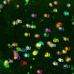
As part of the automated pipeline processing, individual cells are identified by an automatic ROI drawing feature.

The menu-accessible pipelines are invisible for normal operation, and only key-parameters are shown in the main parameter bar. However, pipelines can be opened for editing and arbitrarily changed.
| Development of the unbiased, absolute mitochondrial membrane potential assay has been supported by: |
 |
Theory Overview